State Space Duality (Mamba-2) Part I - The Model

This series is cross-posted at tridao.me

Since the release of Mamba 6 months ago, we’ve been pleasantly surprised by the overwhelming community response. It’s been incredibly gratifying to see the line of research on efficient sequence models we’ve been pursuing for years really resonate with the machine learning community and take off more than we could have anticipated. We’ve seen an enormous amount of exciting follow-up work, from direct applications (e.g. vision , genomics , graphs , and more) to understanding (e.g. on recall abilities , in-context learning , and formal language expressivity ), and an enormous number of online blogs, tutorials, and videos. We couldn’t be more excited about the direction of this research!

Yet despite its potential so far, we weren’t completely satisfied with the first version of Mamba…

Problem 1 (Understanding)

From a conceptual standpoint, one of the reasons we found SSMs so fascinating is how they just feel fundamental. One way this is exemplified is how they have rich ties to many major paradigms of sequence models. As developed in our earlier works on structured SSMs , they seem to capture the essence of continuous, convolutional, and recurrent sequence models – all wrapped up in a simple and elegant model.

But of course, aside from these, there’s another major sequence model paradigm: variants of the ubiquitous attention mechanism. SSMs always felt somewhat disjoint from attention, and we’ve tried for a while to understand their relationship better.

Question 1: What are the conceptual connections between state space models and attention? Can we combine them?

Problem 2 (Efficiency)

From a computational standpoint, despite the work that went into making Mamba fast (in particular, its hardware-aware selective scan implementation) it’s still much less hardware-efficient than mechanisms such as attention. The missing piece is that modern accelerators such as GPUs and TPUs are highly specialized for matrix multiplications. While this isn’t a problem for inference, which is bottlenecked by somewhat different considerations, this can be a big deal during training time.

Question 2: Can we speed up the training of Mamba models by recasting them as matrix multiplications?

These are the main questions that Mamba-2 – in particular, its new state space model variant – tries to address.

The SSD Model

The main point of the Mamba-2 paper is what we call structured state space duality (SSD), which refers to several things:

The SSD model refers to a specific standalone layer, like attention or an SSM, that can be incorporated into deep neural networks
The SSD framework is a general framework for reasoning about this model (and many more theoretical connections)
The SSD algorithm is an algorithm for computing SSD layers much more efficiently than previous SSMs

The main SSD model or “state space dual model” itself really isn’t so complicated! In this first part of a series of blog posts, we’ll provide a self-contained description of the SSD layer (and Mamba-2) in isolation and how it compares to related models, particularly Mamba-1.

In the next parts of this series, we’ll describe the general framework and theoretical connections, which aren’t necessary to actually use Mamba-2.

The Linear (SSM) Mode

SSD starts from the same set of equations as Mamba:

\[\begin{aligned} h_{t} &= A_t h_{t-1} + B_t x_t \\ y_t &= C_t^{\top} h_t \end{aligned}\]

\begin{equation} \label{eq:ssm} (\text{Selective state space model (SSM)}) \end{equation}

To recap, a structured state space model (SSM) defines a map from $x \in \mathbb{R}^\mathtt{T} \to y \in \mathbb{R}^\mathtt{T}$. Think of $x_t$ and $y_t$ as being scalars, and the hidden state $h_t$ as an $\mathtt{N}$-dimensional vector, where $\mathtt{N}$ is an independent hyperparameter called the state size, state dimension, or state expansion factor.

A selective state space model allows the $(A, B, C)$ SSM parameters to vary across time . We’ll think of them as tensors with shapes $A \in \mathbb{R}^\mathtt{(T, N, N)}$, $B \in \mathbb{R}^\mathtt{(T, N)}$, and $C \in \mathbb{R}^\mathtt{(T, N)}$ respectively.As with Mamba-1, we take everything over the reals $\mathbb{R}$, although complex variants as with other structured SSMs like the S4 lineage are also possible.

Structured SSMs require $A$ to have structure to be efficiently computable, such as the most commonly used diagonal structure . In this case $A$ has shape $\mathtt{(T, N)}$ where only the diagonal elements of the $\mathtt{N} \times \mathtt{N}$ matrices are stored.

SSD: Scalar Structured SSM

The original Mamba (or more precisely its core “S6” layer) is exactly a selective SSM with diagonal structure.

The SSD layer of Mamba-2 makes only one small modification: it restricts the diagonal $A$ even further to a scalar times identity structure; in other words the diagonal elements of $A$ must all be the same value. In this case $A$ can be represented with shape just $\mathtt{(T)}$ and one can also identify $A_t$ as just a scalar (and so we’ll sometimes denote it $a_t$).

Multihead SSMs

Equation \eqref{eq:ssm} is defined only for a single dimensional input $x \in \mathbb{R}^\mathtt{T}$. If $X \in \mathbb{R}^\mathtt{(T, P)}$ has $\mathtt{P}$ separate channels, we can use the same dynamics (i.e. the same SSM $(A, B, C)$) independently for each channel. This can be interpreted as a single head of the SSM model.

Here, we think of $X$ as a tensor of shape $\mathtt{(T, P)}$ where $\mathtt{T}$ is the sequence (time) dimension and $\mathtt{P}$ is the “head dimension”.Normally there's an additional batch dimension $\mathtt{B}$ when implementing these models, which we'll ignore throughout this presentation.

Multiple heads can be constructed completely independently; for the remainder of this post, we assume that we’re working with a single head. Note that these heads are exactly analogous to how heads in multi-head attention models work, and in Mamba-2 we also choose similar dimensions as modern Transformers, e.g. $\mathtt{P} = 64$ or $\mathtt{P}=128$. (To scale to larger model widths $\mathtt{D} = \mathtt{d\_model}$, we keep this fixed and increase the number of independent heads.)

We can notate the general (selective) state space model as \begin{equation} \label{eq:ssm-transformation} Y^\mathtt{(T,P)} = \mathsf{SSM}(A^\mathtt{(T,…)}, B^\mathtt{(T,N)}, C^\mathtt{(T,N)})(X^\mathtt{(T,P)}) \end{equation}

Some axes of variation include

The structure on $A$, which affects its parameter shape:
- ... = (N,N) for general (unstructured) SSMs
- ... = (N) for diagonal SSMs (or other structures, such as diagonal-plus-low-rank )
- ... = () for scalar SSMs (i.e. SSD)
The state dimension $\mathtt{N}$ (i.e. d_state)
The head dimension $\mathtt{P}$ (i.e. d_head)

There are other axes of variation of structured SSMs (e.g. time-invariance vs. selectivity, SISO vs. MIMO, real vs. complex, etc.), but we’re highlighting these so that we can contrast Mamba-2 to Mamba-1 in just a second…

The Quadratic (Attention) Mode

But first, let’s switch tacks and forget about state space models for a moment. Given the same tensors above with the same shapes $(A^\mathtt{(T)}, B^\mathtt{(T, N)}, C^\mathtt{(T, N)})$, let’s define a different object.

First, we’ll define the following matrix (don’t worry, we’ll explain more and give it a name in Part II of this series!)

\[L = \begin{bmatrix} 1 & \\ a_1 & 1 & \\ a_2a_1 & a_2 & 1 \\ \vdots & \vdots & \ddots & \ddots \\ a_{\mathtt{T}-1}\dots a_1 & a_{\mathtt{T}-1}\dots a_2 & \dots & a_{\mathtt{T}-1} & 1 \\ \end{bmatrix} .\]

Then, let’s define the following matrix

\begin{equation} \label{eq:ssd-attention} M = L \circ C B^\top \in \mathbb{R}^{\mathtt{(T,T)}} \end{equation}

Finally, $M$ encodes a sequence transformation $x \in \mathbb{R}^\mathtt{T} \to y \in \mathbb{R}^\mathtt{T}$ mapping a 1D input to a 1D output—just as in equation \eqref{eq:ssm}—through basic matrix multiplication $y = Mx$.

What’s special about this? Well, you may notice that it looks very similar to an attention computation. In fact, if all $a_t = 1$, then $L$ is simply the lower-triangular causal mask and \eqref{eq:ssd-attention} is equivalent to causal linear attention :

\[Y = (L \circ Q K^\top) V\]

This is exactly the same as equation \eqref{eq:ssd-attention} if we rename $(C, B, X) \mapsto (Q, K, V)$!

State Space Duality

The so-called “duality” refers to the fact that the two models defined in equations \eqref{eq:ssm} (for the scalar-identity structured $A_t$ case) and \eqref{eq:ssd-attention} are actually exactly the same model, which we can view as a particular function

\[(A^\mathtt{(T)}, B^\mathtt{(T, N)}, C^\mathtt{(T, N)}, X^\mathtt{(T, P)}) \mapsto Y^\mathtt{(T, P)}\]

In the general SSD Framework (Part II of this series), we’ll show this equivalence in two completely different ways, both of which are actually much more general and each quite illuminating.

If you take our word for it, though, then SSD is relatively simple to contrast in relation to either SSMs or attention.

SSD vs. State Space Models

Compared to previous SSMs, SSD is pretty much the same as the core layer of Mamba but with even more structure on the recurrent $A$ matrices.

Mamba-1 (S6) uses diagonal structure on $A$, while Mamba-2 (SSD) uses scalar-times-identity structure on $A$.
Mamba-1 has a head dimension of $\mathtt{P}=1$ (i.e. all channels are completely independently controlled by separate SSMs), while Mamba-2 uses a head dimension of $\mathtt{P}>1$ (something like $\mathtt{P}=64$ by default).

In particular, this can be viewed as weight-tied in two ways:

By restricting the diagonal structure of $A$ to scalar-times-identity, the recurrence dynamics are shared across all $\mathtt{N}$ elements of the state space.
These dynamics are also shared across all $\mathtt{P}$ channels of a given head.

In other words, a single SSM head has total state size $\mathtt{P} \times \mathtt{N}$, which are each governed by separate scalar recurrences in Mamba-1 but are controlled by a single shared recurrence in Mamba-2.

Why make these restrictions? The main motivation is efficiency: these changes are necessary to be able to view the model in its [dual attention form], which allows matrix multiplications to be used.

The Bottom Line: Mamba-1 vs. Mamba-2

Compared to Mamba-1, Mamba-2 allows much larger state dimensions (from N=16 in Mamba-1 to N=64 to N=256 or even higher in Mamba-2) while simultaneously being much faster during training.

But can this hurt us? There’s some intuition to believe that it shouldn’t. One of the main reasons for the selectivity (e.g. $A$ that depends on the input $X$) introduced in Mamba is to let the SSM be able to control whether to remember or ignore particular pieces of information; for example, if a filler “um” is encountered in a text transcript. But if such information should be ignored, then the entire state can ignore it together, and so it should be okay if the state’s dynamics are shared across all features.

Empirically, we haven’t found evidence that the restricted expressivity of Mamba-2 might hurt, but the jury’s still out! From one perspective, Mamba-2 isn’t strictly better than Mamba-1: while it’s a dramatic improvement from a training perspective, Mamba-1 might be better from a pure inference perspective. Since inference speed of SSMs is entirely governed by the state dimension, if one wants to maximize performance for a target inference efficiency (i.e. for a particular state size $\mathtt{N}$), then the increased expressivity of Mamba-1 might be better. We haven’t fully analyzed the (theoretical or empirical) tradeoffs here, and think this would be a cool direction for the community to dig in more!

SSD vs. Attention

Compared, to standard (self-)attention, SSD also only has two differences:

The softmax normalization is dropped.
A separate elementwise mask matrix is applied multiplicatively.

The first difference can be interpreted as what reduces the effective state size of the model from linear to constant, and improves its efficiency from quadratic to linear.

The second difference is what distinguishes SSD from standard linear attention. One way to think of the mask is as input-dependent relative positional encodings. Because of the mask $L$ in \eqref{eq:ssd-attention}, the standard attention score $\langle Q_i, K_j \rangle$ is attenuated by a weight

\[a_{i:j}^\times = a_i \cdots a_{j+1}\]

which can be interpreted as a “discount factor” based on how far apart the positions $i$ and $j$ are. (This interpretation was concurrently espoused by Tobias Katsch’s GateLoop paper.) In its attention form, this input-dependent positional mask can be interpreted as the key factor that encodes the “selectivity” of Mamba!

Best of Both Worlds

So why do we care that there are two views of this model? Well, first of all, it’s extremely mathematically interesting, as we’ll cover in Part II, and we hope will inspire future directions. But there are immediate practical benefits too!

Efficiency: the SSM and Attention Modes

The SSM \eqref{eq:ssm} and attention \eqref{eq:ssd-attention} modes represent two different ways of computing the same function, so let’s contrast them.

First, remember that one main reason why SSMs are interesting to begin with is because computing \eqref{eq:ssm} as a recurrence requires maintaining a constant-size state (size $\mathtt{N}$ per channel) and scales linearly in the sequence length $\mathtt{T}$. The downside is that the raw FLOPs don’t reflect actual speed in practice because of hardware considerations…

On the other hand, computing this sequence transformation $y = Mx$ through equation \eqref{eq:ssd-attention} takes quadratic time in the sequence length, because we’re materializing this $\mathtt{T} \times \mathtt{T}$ matrix. But it can be fast in practice because it only uses matrix multiplications, which are extremely optimized on GPUs and TPUs.

Efficiency: the SSD Mode

So if there are two equivalent ways of computing the same model, when should we use one mode or the other? During inference, there’s no trade-off: the SSM mode is designed for fast autoregressive inference. But what about training? Here there’s a tension between FLOPs and hardware efficiency where the attention mode uses more FLOPs, but uses them more efficiently through matrix multiplications.

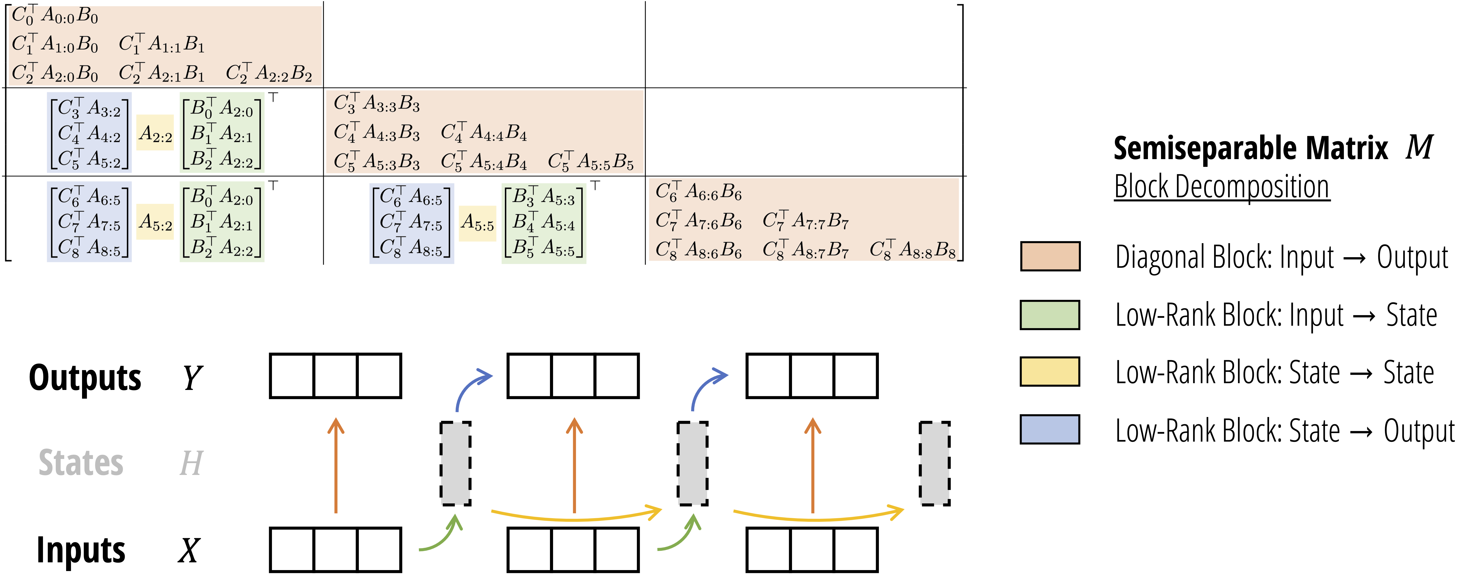
It turns out we can get the best of both worlds by combining the algorithms! There are two equivalent interpretations of this “state space dual” algorithm, either as

A block decomposition of a particular structured matrix that defines the SSD “token-mixing” sequence transformation.
A “chunkwise” algorithm that splits the sequence into segments, computes the quadratic attention form on each segment, and adjusts the result by passing the SSM states between segments.

We’ll leave the details of this algorithm to Part III (or Section 6 of the full paper), as it requires a bit of machinery from the theory to derive. But we do emphasize that the implementation of this algorithm isn’t too complicated – a minimal implementation that we provide is only ~30 lines of PyTorch!

The benefits of the SSD algorithm is that it preserves the same efficient FLOP counts as SSMs (compared to quadratic attention), and also dramatically speeds up training compared to general state space models by utilizing matmuls.

	Attention	SSM	SSD
State size	$\mathrm{T}$	$\mathbf{N}$	$\mathbf{N}$
Training FLOPs	$\mathrm{T}^2\mathrm{N}$	$\mathbf{TN^2}$	$\mathbf{TN^2}$
Inference FLOPs	$\mathrm{T}\mathrm{N}$	$\mathbf{N^2}$	$\mathbf{N^2}$
(Naive) memory	$\mathrm{T}^2$	$\mathrm{TN}^2$	$\mathbf{TN}$
Matrix multiplications?

The Mamba-2 Architecture

Although the core contribution of Mamba-2 is the new SSD layer and theory, we also make some small changes to Mamba’s neural network architecture.

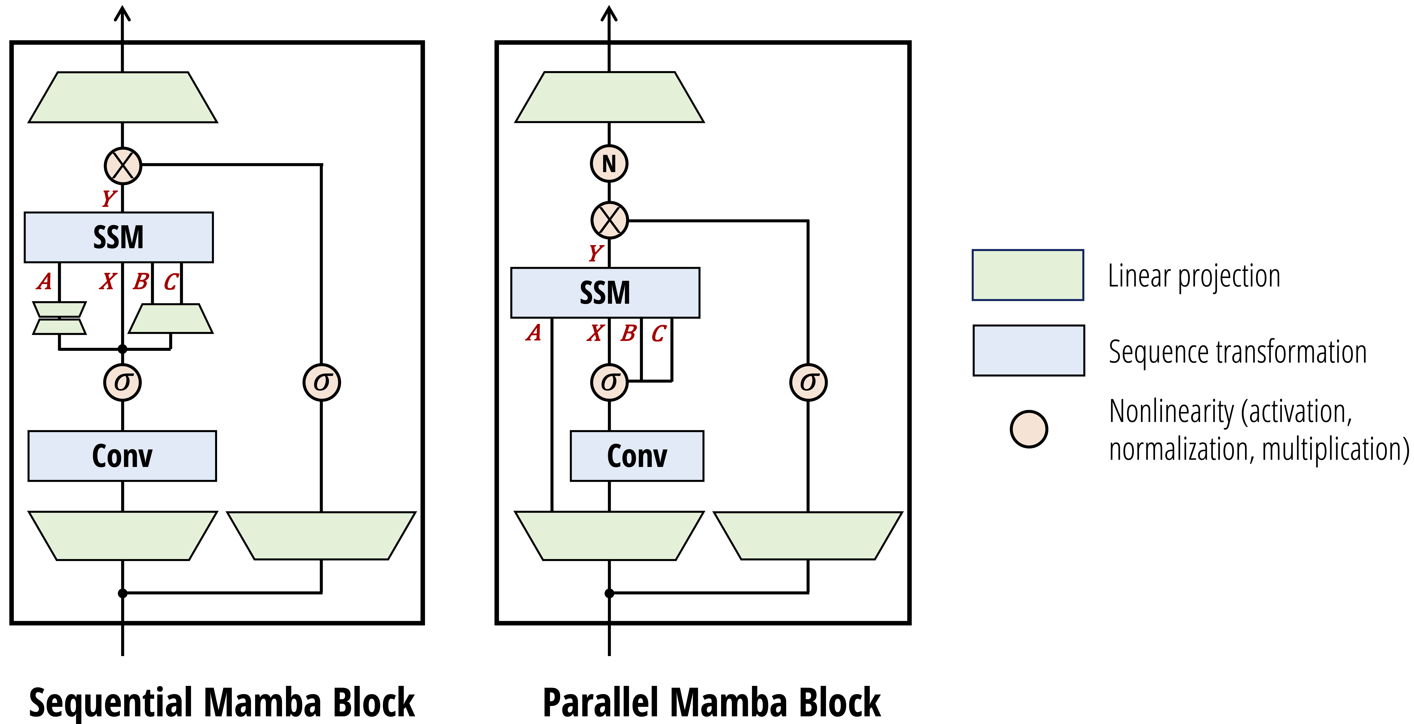
The main change is producing the $(A, B, C)$ SSM parameters in parallel with the $X$ input, instead of sequentially. This is partly motivated by the connections to attention; but more pragmatically, it’s simpler and more amenable to scaling techniques such as tensor parallelism, which will be discussed in Part IV of this series!

There are some other small differences which are covered in more detail in the paper. However, we do want to emphasize that these architectural changes aren’t really the main point of the model.

Language Modeling

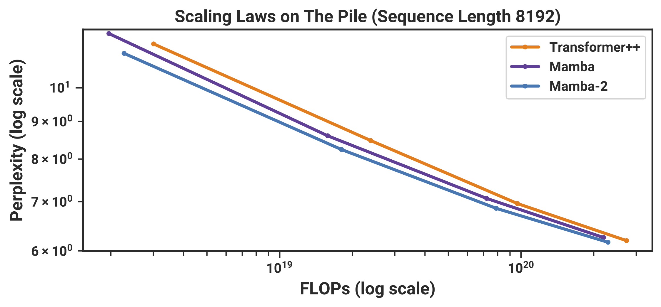
In terms of empirical results, we didn’t test Mamba-2 as extensively as Mamba-1, but believe it should generally be on par or better across the board. Our full language model results use the same protocol as Mamba, and found slightly better scaling at Chinchilla laws .

Fully trained models on the Pile dataset and the standard zero-shot downstream evaluations show similar trends. We emphasize that even when the performance is comparable, Mamba-2 is much faster to train than Mamba-1!

Synthetic Language Modeling: MQAR

More interestingly, we highlight the one synthetic task we tried. Since the original Mamba paper, which investigated synthetics such as Synthetic Copying and Induction Heads, many follow-up works have begun investigating harder associative recall tasks. The multi-query associative recall (MQAR) task introduced by the Zoology and Based line of work has become a de facto standard.

We ran a version of this task that’s much harder than the one usually reported in the literature, and found that Mamba-2 is substantially better than Mamba-1. One reason for the improved performance is the much larger state size (up to $16\times$ larger than Mamba-1 here), which was one of the primary motivations of Mamba-2 in the first place.

Interestingly, Mamba-2 also appears to be noticeably better than Mamba-1 on this particular task even when the state size is controlled. We’re not quite sure why to be honest, and it would be great to ablate the other aspects of the model to investigate… for example, could it be possible that the [restricted structure of SSD] is actually helpful here?

Next Up

In the next part of this series, we’ll go more into the full SSD framework, including how to prove the claimed “duality” of the SSD layer, and strong generalizations of it.